Shoreline roughness of a perfect half-circle

The shoreline roughness metric has been applied to quantify growth patterns of natural and numerical deltas. The metric arises from the fact that a delta shoreline intrinsically bounds a delta area, so the two are related:

\[R = L_{shore} / \sqrt{A_{land}}\]

For the same delta area, a shoreline that is longer would take more turns and be less straight; this indicates a higher shoreline roughness. The intuition of shoreline roughness derives from the ratio of a circle’s circumference and area with increasing radius; the shoreline roughness of a perfect circle is a null value to compare delta data against.

In this guide, we will cover how to create masks directly from an array, and what the value shoreline roughness is for a perfect circle.

Theory for a perfect half-circle

The area of a half circle is given:

\[A = (1/2)~\pi r^2\]

The circumference of a half circle is given:

\[P = \pi r\]

Establish values for the radius \(r\), and evaluate the shoreline roughness metric directly:

r = np.linspace(1, 1000, num=50)
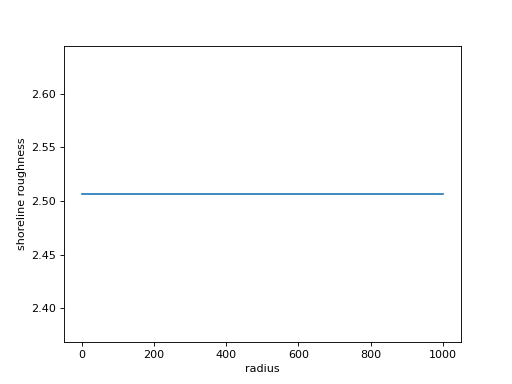
R = (np.pi * r) / np.sqrt(0.5 * np.pi * r * r)

fig, ax = plt.subplots()
ax.plot(r, R)
ax.set_xlabel('radius')
ax.set_ylabel('shoreline roughness')
plt.show()

(Source code, png, hires.png)

The value of the shoreline roughness is not a function of delta radius; it is a scale invariant metric! The theoretical shoreline roughness for a perfect half-circle is approximately 2.506.

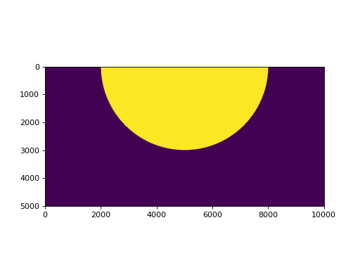
A perfect half-circle rasterized

hcirc = np.zeros((500, 1000), dtype=bool)
dx = 10
x, y = np.meshgrid(
    np.linspace(0, dx*hcirc.shape[1], num=hcirc.shape[1]),
    np.linspace(0, dx*hcirc.shape[0], num=hcirc.shape[0]))
center = (0, 5000)

dists = (np.sqrt((y - center[0])**2 +
                 (x - center[1])**2))
dists_flat = dists.flatten()

# apply the landscape change inside the domain
in_idx = np.where(dists_flat <= 3000)[0]
hcirc.flat[in_idx] = True

fig, ax = plt.subplots()
ax.imshow(hcirc, extent=[x.min(), x.max(), y.max(), y.min()])
plt.show()

(Source code, png, hires.png)

Instantiating masks directly can be done as follows.

lm0 = dm.mask.LandMask.from_array(
    hcirc)
em0 = dm.mask.ElevationMask.from_array(
    hcirc)
sm0 = dm.mask.ShorelineMask.from_mask(
    em0)

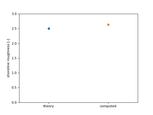
rgh0 = dm.plan.compute_shoreline_roughness(sm0, lm0)

(Source code)

fig, ax = plt.subplots()
ax.plot(0, R[0], 'o')
ax.plot(1, rgh0, 'o')
ax.set_xticks([0, 1])
ax.set_xticklabels(['theory', 'computed'])
ax.set_xlim(-0.5, 1.5)
ax.set_ylim(0, 3)
ax.set_ylabel('shoreline roughness [-]')
plt.show()

(Source code, png, hires.png)