Introduction to mobility functions
To use the mobility functions, you need a set of masks covering various time points from the model output. These can be in the form of a list of mask objects, numpy ndarrays, or xarrays. Or these can be 3-D arrays or xarrays arranged with dimensions t-x-y.
For this example a few masks will be generated and put into lists. Then these lists of masks will be used to compute and plot channel mobility metrics.
Calculation of channel and land masks
The first step to quantifying channel mobility is to determine the location
of the land and channels through time. We do this via the calculation of
both deltametrics.mask.LandMask and deltametrics.mask.ChannelMask
objects. These masks are binary representations of the land and channel
locations, respectively. To read more about masking, refer to the Introduction to Masking objects,
Introduction to Planform objects, and Masking operations API
sections of the documentation.
>>> golfcube = dm.sample_data.golf()
>>> channelmask_list = []
>>> landmask_list = []
>>> for i in range(50, 60):
...     landmask_list.append(
...         dm.mask.LandMask(golfcube["eta"][i, ...], elevation_threshold=0)
...     )
...     channelmask_list.append(
...         dm.mask.ChannelMask(
...             golfcube["eta"][i, ...],
...             golfcube["velocity"][i, ...],
...             elevation_threshold=0,
...             flow_threshold=0.3,
...         )
...     )
...
Calculation of mobility metrics
Next the lists of masks are used to calculate channel mobility metrics.
The metrics calculated are the dry fraction, planform overlap, reworking
fraction, and abandoned fraction. These metrics are calculated using the
functions deltametrics.mobility.calculate_channel_decay(),
deltametrics.mobility.calculate_planform_overlap(),
deltametrics.mobility.calculate_reworking_fraction(), and
deltametrics.mobility.calculate_channel_abandonment(), respectively.
All of these function require at least one list of masks, and can take
additional arguments to specify the base values and window size for the
sliding window calculations. For more information on these functions, refer
to the Masking operations API section of
the documentation.
>>> dryfrac = dm.mobility.calculate_channel_decay(
...     channelmask_list, landmask_list, basevalues_idx=[0, 1, 2], window_idx=5
... )
>>> Ophi = dm.mobility.calculate_planform_overlap(
...     channelmask_list, landmask_list, basevalues_idx=[0, 1, 2], window_idx=5
... )
>>> fr = dm.mobility.calculate_reworking_fraction(
...     channelmask_list, landmask_list, basevalues_idx=[0, 1, 2], window_idx=5
... )
>>> PwetA = dm.mobility.calculate_channel_abandonment(
...     channelmask_list, basevalues_idx=[0, 1, 2], window_idx=5
... )
Plotting the mobility metrics
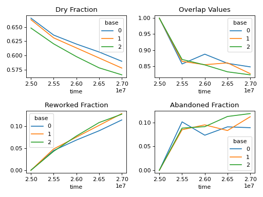
Finally, the mobility metrics are plotted. The metrics are on a single figure below with the dry fraction on the top left, the planform overlap on the top right, the reworking fraction on the bottom left, and the abandoned fraction on the bottom right. The mobility metric for each base time step is plotted in a different color. The base time steps are the first three time steps in the list of masks (per the basevalues_idx argument in the calculation of the mobility metrics). Time is expressed in terms of model seconds, and is known from the Mask objects used to construct the list of masks passed to the mobility functions.
>>> fig, ax = plt.subplots(2, 2)
>>> dryfrac.plot.line(x="time", ax=ax[0, 0])
>>> ax[0, 0].set_title("Dry Fraction")
>>> Ophi.plot.line(x="time", ax=ax[0, 1])
>>> ax[0, 1].set_title("Overlap Values")
>>> fr.plot.line(x="time", ax=ax[1, 0])
>>> ax[1, 0].set_title("Reworked Fraction")
>>> PwetA.plot.line(x="time", ax=ax[1, 1])
>>> ax[1, 1].set_title("Abandoned Fraction")
>>> plt.tight_layout()
>>> plt.show()
(Source code, png, hires.png)
